


【ADHD血液診断】次元削減
目次
0. はじめに
本記事は、以下の記事の続きになります。
https://www.bioinforest.com/adhd1-1
1. サンプル情報の追加
ライブラリをimportし、サンプル情報のファイルを読み込みます。
Text
import timeimport pickle
import pandas as pdimport numpy as np
import matplotlib.pyplot as pltimport seaborn as sns
from scipy.stats import pearsonrfrom sklearn.decomposition import PCAfrom sklearn.manifold import TSNEimport umapfrom scipy.sparse.csgraph import connected_components
import warningswarnings.filterwarnings('ignore')
df_sample = pd.read_csv("src/GSE159104_samples.txt", sep="\t")df_sample| Sample Name | Pair grouping | Twin Status | ADHD_Status | Channel | High Quality Reads | |
|---|---|---|---|---|---|---|
| 0 | RNABL30041_ADHD_rep1 | 31 | clean discordant | ADHD | P14.2016-08-30T13_45_39.0220160891013.fc2.ch15 | 495203 |
| 1 | RNABL30041_ADHD_rep2 | 31 | clean discordant | ADHD | P13.2016-10-21T13_04_11.0234062861006.fc2.ch21 | 2164087 |
| 2 | RNABL30042_CTRL_rep1 | 31 | clean discordant | CTRL | P14.2016-08-30T13_45_39.0220160891013.fc2.ch16 | 1024974 |
| 3 | RNABL30042_CTRL_rep2 | 31 | clean discordant | CTRL | P13.2016-10-21T13_04_11.0234062861006.fc2.ch22 | 2295331 |
| 4 | RNABL30051_CTRL_rep1 | 21 | clean discordant | CTRL | P13.2016-11-22T13_16_36.0234063021020.fc2.ch15 | 69296 |
| ... | ... | ... | ... | ... | ... | ... |
| 149 | RNABL2044_CTRL_rep3 | NaN | NaN | CTRL | P13.2016-04-22T14_16_47.0220160891008.fc2.ch18 | 355566 |
| 150 | RNABL2050_CTRL_rep3 | NaN | NaN | CTRL | P13.2016-04-22T14_16_47.0220160891008.fc2.ch24 | 217718 |
| 151 | RNABL2000_CTRL | NaN | NaN | CTRL | P13.2016-05-31T15_11_07.1231461441002.fc1.ch1 | 189097 |
| 152 | RNABL2057_CTRL_rep3 | NaN | NaN | CTRL | P14.2016-06-07T15_56_34.0231461441003.fc1.ch17 | 189204 |
| 153 | RNABL2058_CTRL_rep2 | NaN | NaN | CTRL | P14.2016-06-07T15_56_34.0231461441003.fc1.ch19 | 227166 |
サンプル情報をyとして列に加えます。
Text
table = {}
for i in range(df_sample.shape[0]): if df_sample["ADHD_Status"][i] == "CTRL": table[df_sample["Channel"][i]] = 0 else: table[df_sample["Channel"][i]] = 1
v = [table[s] for s in df_std.index.tolist()]df_xy = df_stddf_xy["y"] = v
df_xy| GLYCTK-AS1 | RN7SL762P | KDM8 | ... | TNFSF10 | y | |
|---|---|---|---|---|---|---|
| P14.2016-03-31T12_40_25.0220160771004.fc1.ch8 | 1.468904 | 6.854884 | 1.958538 | 0.979269 | 19.789397 | 1 |
| P14.2016-03-31T12_40_25.0220160771004.fc1.ch10 | 0.837903 | 7.541126 | 5.027417 | 4.189514 | 25.137086 | 1 |
| P14.2016-03-31T12_40_25.0220160771004.fc1.ch12 | 0 | 5.632148 | 5.632148 | 8.448221 | 20.103638 | 1 |
| P14.2016-03-31T12_40_25.0220160771004.fc1.ch15 | 2.700708 | 13.503541 | 0.900236 | 2.700708 | 22.505902 | 1 |
| P14.2016-03-31T12_40_25.0220160771004.fc1.ch19 | 2.559553 | 20.476422 | 0 | 0 | 25.168936 | 1 |
| ... | ... | ... | ... | ... | ... | ... |
| P13.2016-11-22T13_16_36.0234063021020.fc2.ch11 | 0 | 9.755917 | 1.393702 | 0 | 38.036464 | 0 |
| P13.2016-11-22T13_16_36.0234063021020.fc2.ch15 | 0 | 0 | 0 | 0 | 42.685478 | 0 |
| P13.2016-11-22T13_16_36.0234063021020.fc2.ch24 | 0 | 38.228511 | 2.012027 | 6.036081 | 17.940573 | 1 |
| P13.2016-12-08T21_33_13.0249463261006.fc2.ch17 | 0 | 71.393385 | 0 | 0 | 11.898897 | 0 |
| P13.2016-12-08T21_33_13.0249463261006.fc2.ch18 | 0 | 63.391107 | 0 | 0 | 8.80432 | 0 |
2. 標準化
Text
x = df_xy.iloc[:, :-1]x_scaled = (x - x.mean()) / x.std()3. PCA
まずは次元削減を実施し、現在のデータのまま十分にADHDであるか判定できそうか大雑把に調べます。
PCA、tSNE、UMAPの順に試していきます。
Text
pca = PCA()pca.fit(x_scaled)
score = pd.DataFrame(pca.transform(x_scaled), index=x_scaled.index)
plt.scatter(score.iloc[:, 0], score.iloc[:, 1], c=df_xy.iloc[:, -1], cmap=plt.get_cmap('jet'))clb = plt.colorbar()clb.set_label('ADHD Status', labelpad=-20, y=1.1, rotation=0)plt.xlabel('PC1')plt.ylabel('PC2')plt.show()
Text
# 寄与率contribution_ratios = pd.DataFrame(pca.explained_variance_ratio_)cumulative_contribution_ratios = contribution_ratios.cumsum()
cont_cumcont_ratios = pd.concat([contribution_ratios, cumulative_contribution_ratios], axis=1).Tcont_cumcont_ratios.index = ['contribution_ratio', 'cumulative_contribution_ratio'] # 行の名前を変更# 寄与率を棒グラフで、累積寄与率を線で入れたプロット図を重ねて描画x_axis = range(1, contribution_ratios.shape[0] + 1) # 1 から成分数までの整数が x 軸の値plt.rcParams['font.size'] = 18plt.bar(x_axis, contribution_ratios.iloc[:, 0], align='center') # 寄与率の棒グラフplt.plot(x_axis, cumulative_contribution_ratios.iloc[:, 0], 'r.-') # 累積寄与率の線を入れたプロット図plt.xlabel('Number of principal components') # 横軸の名前plt.ylabel('Contribution ratio(blue),\nCumulative contribution ratio(red)') # 縦軸の名前。\n で改行していますplt.show()
4. tSNE
Text
tsne = TSNE(n_components=2, random_state=42)corrdinates = pd.DataFrame(tsne.fit_transform(x_scaled))
plt.scatter(corrdinates.iloc[:, 0], corrdinates.iloc[:, 1], c=df_xy.iloc[:, -1], cmap=plt.get_cmap('jet'))clb = plt.colorbar()clb.set_label('ADHD Status', labelpad=-20, y=1.1, rotation=0)plt.xlabel('tSNE 1')plt.ylabel('tSNE 2')plt.show()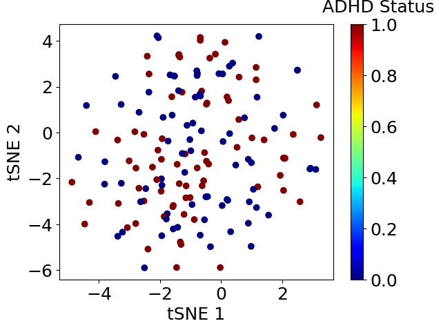
5. UMAP
Text
embedding = pd.DataFrame(umap.UMAP().fit_transform(x_scaled))
plt.scatter(embedding.iloc[:, 0], embedding.iloc[:, 1], c=df_xy.iloc[:, -1], cmap=plt.get_cmap('jet'))clb = plt.colorbar()clb.set_label('ADHD Status', labelpad=-20, y=1.1, rotation=0)plt.xlabel('UMAP 1')plt.ylabel('UMAP 2')plt.show()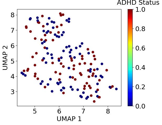
6. まとめ
次元削減を実施したところ、ADHD患者と健常人はうまく分かれませんでした。
このまま機械学習のモデルを作成しても、通常はうまい判別モデルはできません。
モデル作成の前に一工夫する必要がありそうです。